Transformers: From Understanding Language to Generating Text

Hi everyone. Today we’ll learn about Transformers.

We’ll understand what a Transformer is, why it came, who introduced it, what it does, and actually how it does it.

So let’s start.

---

1. Prerequisite: How Do We Represent Language?

Before understanding the Transformer, we first need to understand what we actually give as input to it.

We know that a computer needs a numerical representation. It can’t understand raw text as input in the same way humans do.

So what input do we give to the Transformer?

Suppose, for our example, we have a raw string:

“I love cats.”

We need to convert this into a numerical representation.

Tokenization

For this, we use tokenization.

Tokenization breaks the raw text into smaller pieces called tokens.

For our example:

"I love cats"
      ↓
["I", "love", "cats"]

Each token has its own unique integer ID.

For example:

"I"     → 12
"love"  → 45
"cats"  → 87

These IDs don’t have any meaningful value by themselves. They are simply identifiers for the tokens in the model’s vocabulary.

Embeddings

The model has an embedding matrix that contains a vector representation for each token ID.

So, based on the token ID, we can get its corresponding vector.

For example:

"I"     → [0.2, 0.7, 0.1, 0.4]
"love"  → [0.8, 0.1, 0.6, 0.3]
"cats"  → [0.5, 0.9, 0.2, 0.7]

These are called embeddings.

So the complete process is:

Raw text
   ↓
Tokenization
   ↓
Token IDs
   ↓
Embedding lookup
   ↓
Embedding vectors

Now we have a numerical representation of our input that the neural network can work with.

Embeddings place words into a continuous high-dimensional geometric space where words with similar semantic meanings or syntactic roles end up closer together.

---

2. Why Did We Need Transformers?

Now let’s go back and understand why Transformers came into the picture in the first place.

We start with NLP, which stands for Natural Language Processing.

The basic problem is:

How can a machine process and work with human language?

There are many tasks where we want to do this, such as:

• Translation
• Summarization
• Text generation
• Question answering
• Speech recognition

Earlier, models such as RNNs, or Recurrent Neural Networks, were used to process natural language.

RNNs

Suppose we have:

“I love cats.”

An RNN processes the tokens sequentially, one by one.

"I"
 ↓
RNN
 ↓
memory

"love"
 ↓
RNN + previous memory
 ↓
updated memory

"cats"
 ↓
RNN + previous memory
 ↓
updated memory

The important idea here is that the RNN passes its previous state to the next step.

So the RNN can carry information from previous tokens.

For example, when processing "love", it can use information from "I".

When processing "cats", it can use information from "I" and "love" through its previous state.

So RNNs do have a form of context.

The Problem with RNNs

The difficulty comes with long sequences.

As the sentence becomes longer, information has to travel through many sequential steps, and preserving information from much earlier in the sequence becomes difficult.

This is one of the reasons models such as LSTM, or Long Short-Term Memory, were introduced.

LSTMs introduced mechanisms called gates that helped the model decide what information to keep, what information to forget, and what new information to store.

Then came GRUs, or Gated Recurrent Units, which provided a simpler gated architecture.

But there was still a fundamental issue:

They were still processing the sequence sequentially.

Token 1 → Token 2 → Token 3 → Token 4 → ...

This makes it difficult to process all the tokens in parallel during training.

The Sequential Bottleneck: Because step t strictly depends on the hidden state of step t - 1, RNNs cannot process tokens concurrently across the sequence dimension. On modern GPUs built for massive parallelism, this sequential dependency prevents full hardware utilization.

So we needed a different approach.

We wanted a mechanism where tokens could interact with each other while allowing the computation to be performed much more efficiently in parallel.

This is where attention comes into the picture.

And this eventually led to the Transformer.

---

3. The Transformer

In 2017, researchers introduced the Transformer architecture in the paper:

“Attention Is All You Need” (Vaswani et al.)

The Transformer introduced an architecture based heavily on attention mechanisms rather than recurrence.

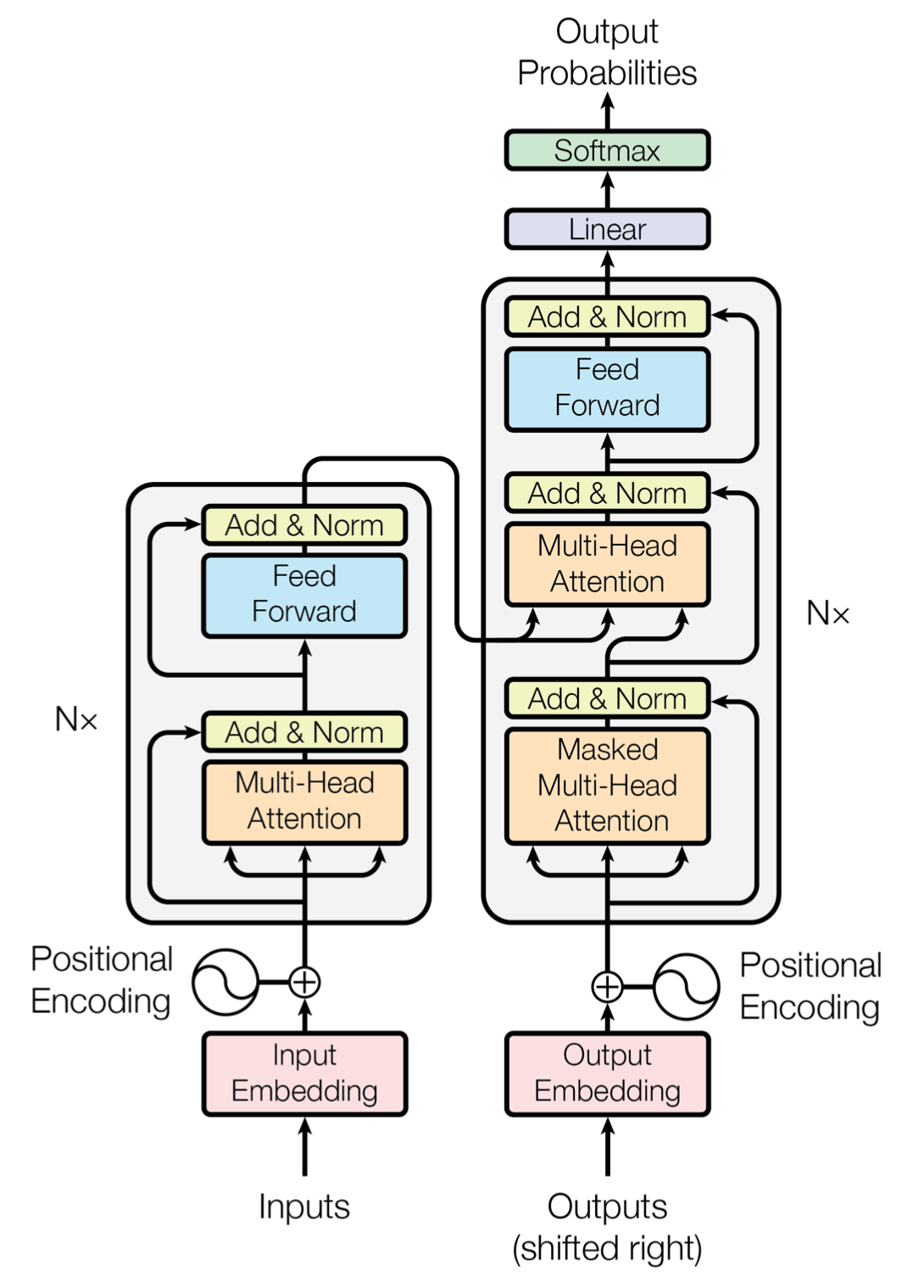
The original Transformer architecture had two major parts:

Encoder
   +
Decoder

The high-level idea is:

Input sentence
      ↓
   Encoder
      ↓
Contextual representation
      ↓
   Decoder
      ↓
Output sentence

For example, we could have a translation task:

"I love cats"
      ↓
   Encoder
      ↓
contextual representation
      ↓
   Decoder
      ↓
"Me encantan los gatos"

The encoder processes the input and creates contextual representations.

The decoder uses that information to generate the output.

But before the Transformer can understand context, we have another problem to solve.

---

4. Why Do We Need Positional Information?

Let’s return to our example:

“I love cats.”

We already converted each token into an embedding.

But embeddings alone don’t tell us where a token appears in the sentence.

Consider:

"I love cats"

and:

"cats love I"

They contain the exact same tokens, but the order is completely different.

The model needs information about the position of each token.

Therefore, conceptually, the Transformer input contains:

Token embedding
      +
Positional information
      ↓
Transformer input

The positional information tells the model where each token occurs in the sequence.

Because Transformers process all tokens simultaneously rather than one-by-one, they have zero inherent sense of order. Positional encodings (either fixed sinusoidal waves or learned vectors) are added directly to the token embeddings to inject sequence order without changing vector dimensions.

Now we have numerical representations that contain both:

• Information about the token itself
• Information about its position

But there is still another important problem.

The embedding of "bank" should somehow behave differently in:

“I deposited money in the bank.”

and:

“I sat beside the river bank.”

The model needs to understand the relationship between a token and the other tokens around it.

This is where self-attention comes in.

---

5. How Does the Transformer Understand Context?

Now let’s move to the most important part of the Transformer:

Self-Attention

The question we want to answer is:

How does one token know which other tokens are important to it?

Again, we’ll use our same example:

“I love cats.”

We want each token to be able to look at the other tokens and determine how relevant they are.

For example, when processing "cats", the model can consider "I" and "love" as well.

So the basic idea is:

Input vectors
     ↓
Self-Attention
     ↓
Contextual representations

But how does self-attention actually work?

This is where Query, Key, and Value, or Q, K, and V, come in.

Query, Key, and Value

During training, the model learns three weight matrices:

WQ
WK
WV

These are learned parameters of the model.

We use them with our input vectors to calculate:

Input
  ↓
 ┌──────┬──────┬──────┐
 ↓      ↓      ↓
WQ     WK     WV
 ↓      ↓      ↓
Q      K      V

So Q, K, and V are not the learned matrices themselves. They are the vectors calculated from the input using the learned matrices.

Conceptually think of them as a search retrieval system:

• Query ($Q$): “What information am I looking for?”
• Key ($K$): “What kind of information does this token contain for matching?”
• Value ($V$): “What information should I actually take from this token?”

Now we have Q, K, and V for our tokens.

Attention Scores

Next, we want to know how strongly each token should pay attention to the other tokens.

For this, we compare the Query of a token with the Keys of all tokens via a dot product.

Conceptually:

Q × Kᵀ
   ↓
Raw attention scores

This produces a matrix of scores.

The higher the score, the more relevant that token is to the current query.

These raw scores can become large, so we scale them by the square root of the key dimension, √(64) or √(d_k).

In our example, if the key dimension were 64, we would divide by:

√(64) = 8

So:

QKᵀ
 ↓
QKᵀ / √64

Why scale by √(d_k)? When the vector dimension d_k is large, dot products can grow very large in magnitude. Large values push the softmax function into regions where gradients are extremely small (vanishing gradient problem). Scaling by √(d_k) keeps variance around 1 and preserves healthy gradients during training.

Softmax

After scaling the scores, we apply softmax.

Softmax converts the scores into a probability-like distribution whose values sum to 1.

For example:

"I"     → 0.10
"love"  → 0.70
"cats"  → 0.20

Now these are our attention weights.

They tell us how much attention the current token should give to each token.

Applying the Values

Now we use these attention weights with the Value vectors.

Attention weights
        ×
Value vectors
        ↓
Contextual representation

For example, if we are processing "cats", its new representation will contain information gathered from the Value vectors of:

"I"
"love"
"cats"

according to their attention weights.

So the output is no longer just the original "cats" representation.

It is a context-aware representation of "cats".

And this happens for every token in parallel.

That’s self-attention!

---

Interactive Transformer Explorer

Try out the interactive widget below to inspect how tokens map to vectors, and see how the attention weights change when switching from full self-attention to causal masking:

---

6. Multi-Head Attention

Now think about the entire process of calculating attention.

What if we don’t want the model to look at relationships between tokens in only one way?

What if we want it to look at the sentence from multiple perspectives?

That’s where Multi-Head Attention comes in.

Instead of having only one attention mechanism, we have multiple attention heads working in parallel.

Conceptually:

                 Input
                   ↓
       ┌───────────┼───────────┐
       ↓           ↓           ↓
     Head 1      Head 2      Head 3 ...
       ↓           ↓           ↓
 different attention patterns
       └───────────┼───────────┘
                   ↓
                Combine

Each head has its own learned parameters (W_i^Q, W_i^K, W_i^V), so each head can learn different relationships between tokens (such as grammatical relations, semantic relationships, or positional focus).

After all the heads produce their outputs, we concatenate them and project them with a final linear layer:

MultiHead(Q, K, V) = Concat(head_1, ..., head_h) × W_O

The original Transformer used 8 attention heads.

---

7. What Happens After Attention?

So far, we have performed multi-head self-attention and obtained contextual representations.

But that’s not the end of the encoder layer.

We still have more operations.

The complete encoder layer consists of:

Input
  ↓
Multi-Head Self-Attention
  ↓
Add + Layer Normalization
  ↓
Feed-Forward Network
  ↓
Add + Layer Normalization
  ↓
Output

Add + Layer Normalization

First, we perform the Add operation.

The idea is to add the original input to the output of the attention layer:

Output = LayerNorm(x + Sublayer(x))

The original information is therefore able to flow forward instead of being completely replaced by the transformed representation.

This is called a residual connection.

Then we apply Layer Normalization.

So conceptually:

Original input
      +
Attention output
      ↓
Layer Normalization

Feed-Forward Network

Next comes the Feed-Forward Network (FFN).

This is a small neural network with two linear transformations and a non-linear activation function (like ReLU or GELU) in between:

FFN(x) = max(0, xW_1 + b_1)W_2 + b_2

The important point is that it operates on each token representation individually and identically.

So:

Contextual token representations
             ↓
      Feed-Forward Network
             ↓
   transformed representations

After that, we again perform:

Add
 ↓
Layer Normalization

And now we have the final output of one encoder layer.

The Encoder Stack

The Transformer doesn’t use just one encoder layer.

It stacks multiple encoder layers vertically.

In the original 2017 Transformer, there were 6 encoder layers.

Input
 ↓
Encoder Layer 1
 ↓
Encoder Layer 2
 ↓
Encoder Layer 3
 ↓
Encoder Layer 4
 ↓
Encoder Layer 5
 ↓
Encoder Layer 6
 ↓
Encoder Output

The output of one encoder layer becomes the input to the next one.

As the representation passes through these layers, the model builds increasingly rich, abstract representations of the input sentence.

---

8. The Decoder: How Do We Generate the Output?

Now let’s move to the decoder.

Remember our original translation task:

English:
"I love cats"
      ↓
   Encoder
      ↓
contextual representation
      ↓
   Decoder
      ↓
Spanish:
"Me encantan los gatos"

The encoder has processed the input.

Now the decoder has to generate the output.

The decoder generates the output token by token (autoregressively):

Step 1: Me
          ↓
Step 2: Me encantan
          ↓
Step 3: Me encantan los
          ↓
Step 4: Me encantan los gatos

At every step, it uses the tokens generated so far to predict the next token.

Masked Multi-Head Self-Attention

The first major component of the decoder is masked multi-head self-attention.

Why do we need a mask?

Suppose the decoder is trying to predict:

Me encantan

It should not be allowed to look at future tokens such as:

los gatos

because those are supposed to be predicted later!

So the mask prevents a token from looking at future positions.

Conceptually:

Me       → can see: [Me]
encantan → can see: [Me, encantan]
los      → can see: [Me, encantan, los]
gatos    → can see: [Me, encantan, los, gatos]

Causal Masking: In training, we feed the entire target sequence at once for parallel training, but we add an upper-triangular mask of -∞ to the attention matrix before softmax. This forces the attention weights for any future positions to 0, ensuring token i can only attend to positions ≤ i.

After masked self-attention, we perform:

Add + Layer Normalization

Cross-Attention

Next comes another attention mechanism called cross-attention (or encoder-decoder attention).

Why is it called cross-attention?

Because now we are connecting two different sources:

Decoder representation
        +
Encoder output

In cross-attention:

• The Query ($Q$) comes from the decoder
• The Key ($K$) and Value ($V$) come from the encoder’s output

Conceptually:

Decoder representation
        ↓
        Q
        │
        │
        ↓
   Cross-Attention
        ↑
        │
   K + V from
   Encoder output

The decoder is essentially asking:

“From the information in the input sentence, what is useful for generating my next output token?”

After cross-attention:

Add + Layer Normalization
        ↓
Feed-Forward Network
        ↓
Add + Layer Normalization

The result is the output of the decoder layer.

Just like the encoder, the original Transformer stacked 6 decoder layers on top of each other.

---

9. From Decoder Output to the Next Token

At this point, the decoder has produced a final numerical representation.

But we don’t want a numerical vector as our final answer.

We want an actual word or token!

So we need to convert the decoder’s output into a probability for every token in the vocabulary.

We do this using a Linear layer followed by Softmax:

Final decoder representation
          ↓
      Linear layer
          ↓
   Vocabulary logits
          ↓
        Softmax
          ↓
Probability of every token in vocabulary

For example, the model might output probabilities:

"gatos"   → 0.72  (72%)
"perros"  → 0.08  (8%)
"libros"  → 0.03  (3%)
...

The model selects the most probable token (or samples from the distribution):

"gatos"

Now that token becomes part of the decoder’s input for the next step.

The autoregressive cycle repeats until the model generates a special <end-of-sequence> (EOS) token:

Me
 ↓
Me encantan
 ↓
Me encantan los
 ↓
Me encantan los gatos
 ↓
<EOS>

---

10. Summary of the Architecture

Here is the complete journey from raw text to generated output:

Input text
    ↓
Tokenization
    ↓
Token IDs
    ↓
Embeddings + Positional Information
    ↓
Encoder Stack (N = 6 layers)
    ├── Multi-Head Self-Attention
    ├── Add & LayerNorm
    ├── Feed-Forward Network
    └── Add & LayerNorm
    ↓
Contextual Representations (K, V)
    ↓
Decoder Stack (N = 6 layers)
    ├── Masked Multi-Head Self-Attention (Q from decoder)
    ├── Add & LayerNorm
    ├── Cross-Attention (Q from decoder, K & V from encoder)
    ├── Add & LayerNorm
    ├── Feed-Forward Network
    └── Add & LayerNorm
    ↓
Linear Layer
    ↓
Softmax
    ↓
Next Token Prediction
    ↓
Repeat until <EOS>

The important thing to understand is that the Transformer isn’t just one single magic trick.

It’s a complete architecture made up of several complementary components, where each component solves a specific problem:

Component	Role in the System
Tokenization	Breaks continuous text into discrete, manageable tokens
Embeddings	Maps discrete tokens into continuous geometric vectors
Positional Information	Restores order information lost due to parallel processing
Self-Attention	Enables every token to dynamically weigh and gather context from other tokens
Multi-Head Attention	Allows the model to attend to information at different positions from multiple representation subspaces
Feed-Forward Network	Applies non-linear transformations to each token representation individually
Encoder	Builds deeply contextualized representations of the input sequence
Decoder	Autoregressively generates output tokens conditioned on the encoder’s context
Masked Attention	Enforces causality so future tokens cannot be seen during generation
Cross-Attention	Bridges the decoder queries with the encoder’s keys and values
Linear + Softmax	Projects hidden vectors onto the vocabulary to output token probabilities

And this is the architecture that became the foundation for virtually all modern large language models, from GPT-4 and Claude to LLaMA and Gemini.